
Recruiter-to-Open-Roles Ratio: How Many Recruiters Your Plan Needs
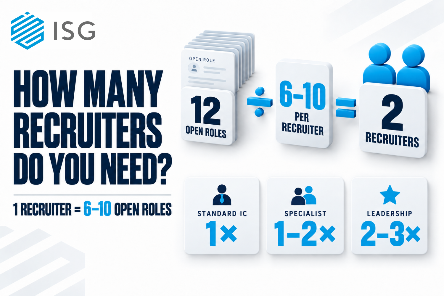
One full-cycle recruiter carries six to ten open roles at a time. That band is the recruiter-to-open-roles ratio, and the ratio sizes every recruiting team. Divide peak parallel requisitions by the band and round up. Role difficulty then weights the count, because a leadership search carries the load of two to three standard requisitions.
Overload announces itself through req aging, reactive sourcing, and slipping feedback. Underload announces itself on the payroll. The ratio decides in-house headcount, embedded capacity, and the ceiling of any hiring plan. We run engagements on the six-to-ten band at ISG Partners, and the full math is below.
What Is the Recruiter-to-Open-Roles Ratio?
The recruiter-to-open-roles ratio measures how many active requisitions one recruiter manages at once. Other names describe the same number: recruiter-to-req ratio, requisition load, recruiter bandwidth. The ratio is the load-bearing number in capacity planning. Every hiring plan silently assumes a ratio. Most plans never write the assumption down.
A plan promising twenty parallel searches to one recruiter fails in the plan, months before failing in the market. Writing the ratio down converts a hope into a staffing decision. The written ratio also gives finance and talent teams one shared number. Capacity debates end faster when both sides read the same math.
How Many Open Roles Can One Recruiter Handle?
One full-cycle recruiter handles six to ten open roles at a time. Full-cycle load explains the band. Each requisition contains sourcing hours, screening calls, interview coordination, offer management, and post-offer follow-through. Six to ten of those workloads fill a professional week.
The band assumes real searches, run properly, with pipelines built rather than borrowed. Recruiters juggling more reqs stop recruiting. They start administrating, and the pipelines show the difference within a month.
What Does Full-Cycle Load Contain?
Full-cycle load contains five workstreams per requisition: sourcing, screening, coordination, offers, and follow-through. Sourcing builds the pipeline before applications arrive. Screening converts the pipeline into a shortlist. Coordination runs the interview loop and keeps every transition dated.
Offer management carries the close, from structure through signature. Follow-through holds the placement steady after the start date. Each workstream consumes real weekly hours. Multiply the hours by six to ten reqs, and the band explains itself.
Why Does the Range Run Six to Ten?
Four factors set a recruiter's position inside the six-to-ten band. Role difficulty moves the number most. Process maturity moves the number next: calibrated scorecards and booked interview slots free recruiter hours.
Market heat matters, because thin candidate markets demand more sourcing per hire. Tooling closes the list. Strong systems push capacity toward ten. Hard searches in hot markets pull capacity toward six. The band is a dial, not a constant.
How Do You Calculate How Many Recruiters You Need?
Three calculations size a recruiting team: forward, backward, and timeline. Each one answers a different planning question. Run all three before committing headcount or capacity.
How Does the Forward Calculation Work?
The forward calculation divides peak parallel roles by the six-to-ten band and rounds up. A plan with fourteen seats open at peak needs two recruiters. Rounding always goes up, because a recruiter and a half does not exist. Peak matters more than total. Forty hires spread evenly across a year never stress capacity.
Fourteen open at once defines the requirement. Find the peak by stacking the plan month by month. The tallest column sets the staffing number. Plans without a stacked view hide their own peaks. The hiring plan the ratio plugs into maps the peaks before the math runs.
How Does the Backward Calculation Work?
The backward calculation multiplies available recruiters by the band to find the plan's ceiling. One recruiter supports six to ten parallel searches, and no plan above the ceiling survives contact with the calendar. Backward math protects companies from optimistic planning. The plan shrinks, the timeline extends, or the capacity grows. No fourth option exists.
How Does the Timeline Calculation Work?
The timeline calculation converts total roles and search lead times into true parallel load. Roles rarely all run at once. Multiply each role by expected search weeks. Divide the total search-weeks by the weeks available. The result is average parallel load, the honest version of the requirement. Sequencing then flattens the peaks.
A plan resequenced by trigger dates often needs one recruiter where the raw count suggested two. A quick example shows the effect. Twelve roles at eight search-weeks each equal 96 search-weeks. Spread across 48 available weeks, the true parallel load is two roles at a time.
How Does Role Difficulty Change the Ratio?
Role difficulty weights the requisition count, because requisitions carry different loads. Counting reqs like they weigh the same breaks more capacity plans than bad math does. The weights we apply are mapped below:
| Role type | Load weight | Why the weight differs |
|---|---|---|
| Executive and leadership search | 2 to 3 units | Stakeholder depth, thin markets, long cycles |
| Specialist individual contributor | 1 to 2 units | Scarce candidate pools, heavy sourcing |
| Standard individual contributor | 1 unit | The baseline the band assumes |
| Volume batch of identical seats | Under 1 unit each | One pipeline feeds many offers |
Weighted counting changes real staffing answers. Eight open reqs containing two executive searches weigh eleven to twelve units. The same eight as an SDR batch weigh five. Same req count, different team size.
Weights also shift during the year. Searches close, new reqs open, and the weighted total moves. Re-run the weighted count monthly, at the same review where the aging column gets read.
How Do You Count Batch Requisitions?
Batch requisitions share one pipeline, so the batch counts as a fraction per seat. Five identical SDR seats run one sourcing motion, one screen standard, one interview loop. The load sits closer to three units than five. The fraction shrinks as the batch grows and the profile stays identical. The fraction snaps back to one the moment seats diverge in level, location, or profile.
What Are the Symptoms of Recruiter Overload?
Overload announces itself through five symptoms: req aging, reactive sourcing, feedback slippage, review theater, and bar drift. Req aging spreads first. Candidates sit past agreed windows across many roles at once, and reading stage aging in weekly reviews catches the spread early. Sourcing turns reactive next: inbound applications replace built pipelines.
Feedback windows slip from days to weeks. Pipeline reviews turn into status recitals with no decisions. The quality bar drifts last and costs most, because tired screens pass tired candidates. Each symptom traces to the same arithmetic. The load exceeded the band, and the work adjusted itself downward.
What Does Underloading Cost?
Underloaded recruiters cost payroll without producing pipeline, and the cost hides better than overload does. Fixed recruiting headcount meets lumpy hiring demand, and the mismatch runs both directions. Hiring waves overload the team.
Quiet quarters idle the team. Flexing recruiting capacity when plans change covers the structural answer: capacity that scales with the plan instead of sitting on the org chart.
Honest capacity planning names both failure modes. A ratio audit that only checks for overload reads half the ledger. Idle months deserve the same scrutiny as crushed ones.
When Do You Hire In-House Recruiters vs Embedded Capacity?
Sustained multi-year volume at full load justifies in-house recruiters, and wave-shaped demand justifies embedded capacity. The ratio makes the decision measurable. Demand holding at six-plus weighted units for years fills an in-house seat honestly.
Demand arriving in waves fits a dial better than a hire. Our embedded model deploys a dedicated recruiter within 48 hours, carries the full six-to-ten load, and steps down month to month when the wave passes.
Fractional capacity sits between the two models, sharing one recruiter across companies at partial load, and how fractional recruiter capacity compares maps that boundary.
Hybrid structures work too. An in-house recruiter carries the steady base. Embedded capacity absorbs the peaks. The ratio math stays identical across every model, which is the point of learning the math. Cost shape separates the models more than capability does. In-house capacity is fixed cost. Embedded capacity is variable cost that follows the plan.
Many clients run embedded first, then convert to an in-house seat once the base load proves stable for a year. We support the transition, because honest capacity planning outlasts any single engagement.
Frequently Asked Questions
What is a good recruiter-to-req ratio?
Six to ten open roles per full-cycle recruiter, weighted by difficulty. Hard searches pull the number toward six. Mature processes push the number toward ten.
How many recruiters per 100 employees?
Headcount ratios mislead, because open-role load decides capacity, not company size. A stable 500-person company needs less recruiting capacity than a 60-person company hiring twenty roles.
How many open roles is too many for one recruiter?
Loads above ten weighted units break full-cycle work. The recruiter stops building pipelines and starts administrating requisitions.
What happens when recruiters are overloaded?
Req aging spreads, sourcing turns reactive, feedback slips, and the quality bar drifts. The symptoms appear in weekly pipeline reviews weeks before the metrics confirm them. Catch the pattern at the review stage and the fix costs a capacity conversation.
How fast can embedded recruiting capacity deploy?
Our embedded model deploys a dedicated recruiter within 48 hours. Most clients see qualified candidates inside the first two to three days.
Key Takeaways: Write the Ratio Down
Recruiting capacity runs on one band: six to ten weighted requisitions per full-cycle recruiter. Run the forward, backward, and timeline calculations.
Weight the reqs by difficulty. Watch the aging column for the first overload signal. Name both failure modes, because idle capacity and crushed capacity cost real money in different columns. The ratio is small math with large consequences.
We size every ISG Partners engagement on the six-to-ten band, from a single senior search through full team builds and executive search. Capacity scales with the plan, deploys within 48 hours, and steps down when the wave passes. Full-cycle recruiting inside our engagements shows what the load contains. Bring your open-roles list to a discovery call, and we run the weighted math together.